To create a ternary plot from origin and insertion data, first we need data. Attachment centroid data are available for the AL_008 specimen of Alligator mississippiensis (although similar data can be extracted directly from stl files; see the “Working with stl files” article).
library(MuscleTernary)
library(ggtern)
library(readr)

AL008 <- read_csv(system.file("extdata",
                              "AL_008_data.csv",
                              package = "MuscleTernary"),
                  show_col_types = FALSE) |>
  dplyr::select(-side)
AL008
#> # A tibble: 18 × 8
#>    muscle x_origin y_origin z_origin x_insertion y_insertion z_insertion  force
#>    <chr>     <dbl>    <dbl>    <dbl>       <dbl>       <dbl>       <dbl>  <dbl>
#>  1 mAMES      87.6     41.6   -168.        109.         4.92      -133.   665.
#>  2 mAMES     -83.8     45.1   -163.       -108.         7.69      -141.   612.
#>  3 mAMEM      34.2     42.8   -140.        103.        -1.59      -129.   272.
#>  4 mAMEM     -30.2     43.4   -139.       -103.         2.88      -144.   298.
#>  5 mAMEP      27.1     65.4   -130.         92.2       -9.95       -71.7   84.5
#>  6 mAMEP     -19.7     69.6   -128.        -90.2       -2.99       -79.1   83.2
#>  7 mAMP       64.2     35.9   -172.        110.       -53.8       -140.  2720.
#>  8 mAMP      -63.6     35.8   -173.       -108.       -51.9       -138.  2713.
#>  9 mPSTs      23.3     68.3   -118.         95.9      -78.9        -17.5  698.
#> 10 mPSTs     -16.9     69.0   -116.        -88.2      -78.5        -11.9  672.
#> 11 mPSTp      19.5     48.9   -119.         97.8      -59.6       -143.    10.8
#> 12 mPSTp     -12.5     48.7   -117.        -92.9      -58.1       -144.    13.3
#> 13 mPTd       38.8     21.3    -68.8        91.0      -28.5       -222.  3643.
#> 14 mPTd      -34.9     20.6    -62.6       -91.5      -26.2       -221.  3819.
#> 15 mPTv       47.8    -50.5   -129.        112.       -21.2       -246.   701.
#> 16 mPTv      -40.9    -47.4   -129.       -114.       -22.1       -239.   694.
#> 17 mDM        76.4     56.2   -206.         86.7        9.90      -255.   674.
#> 18 mDM       -75.5     58.0   -201.        -90.7       13.1       -251.   729.
We need to convert the x, y, and z origin and insertion columns into
relative ternary coordinates using the coords_to_ternary()
function. Here we also use the grouping option to return
the mean for each muscle, because the original data have both left and
right (two rows per muscle; note that the side column was
dropped above).
ternary_coords <- coords_to_ternary(coords = AL008, grouping = "muscle")
ternary_coords
#> # A tibble: 9 × 5
#>   muscle  force     x     y     z
#>   <chr>   <dbl> <dbl> <dbl> <dbl>
#> 1 mAMEM   285.  72.6  26.2   1.13
#> 2 mAMEP    83.9 35.6  42.2  22.2
#> 3 mAMES   638.  19.7  50.2  30.2
#> 4 mAMP   2717.  18.5  71.3  10.2
#> 5 mDM     701.   3.60 44.3  52.1
#> 6 mPSTp    12.1 34.0  62.5   3.49
#> 7 mPSTs   685.  13.9  58.1  28.1
#> 8 mPTd   3731.  10.0   7.92 82.1
#> 9 mPTv    697.  25.8   4.09 70.1
The x, y, and z columns sum to
100 for each row: these represent the percent contributions of each
orthogonal direction to the muscle’s overall orientation.
The force column contains the estimated force for each
muscle. Force can be estimated from PCSA, which can be derived from
attachment areas (see the “Working with stl files” vignette).
The simplest ternary plot simply maps the x,
y, and z columns and colors points by
muscle:
ggtern(data = ternary_coords,
       aes(x = x, y = y, z = z,
           color = muscle)) +
  geom_point()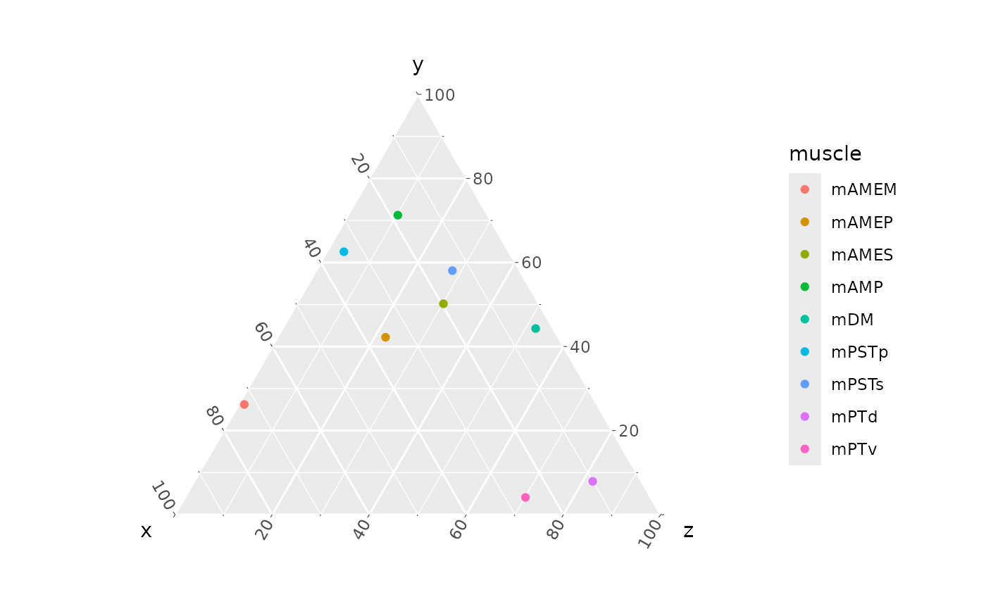
We can make this a more ready-to-use plot by recoloring using the
standard palette for muscle colors. muscle_color_map() is a
function that returns the mapping of muscle to its hex code.
muscle_color_map
#> function ()
#> {
#>     cmap <- ggplot2::scale_color_manual(name = "Muscle", values = c(mAMES = "#0000FF",
#>         mAMEM = "#55FFFF", mAMEP = "#8080FF", mAMP = "#00FF00",
#>         mPSTs = "#FF80FF", mPSTp = "#400080", mPTd = "#FF8000",
#>         mPTv = "#FF0000", mPPt = "#FFC0CB", mDM = "#FF0080",
#>         mLPt = "#09C4A8", mEM = "#FFFF00", mPM = "#7DB7E6"))
#>     return(cmap)
#> }
#> <bytecode: 0x5574c118f128>
#> <environment: namespace:MuscleTernary>

ggtern(data = ternary_coords,
       aes(x = x, y = y, z = z,
           color = muscle)) +
  geom_point() +
  muscle_color_map()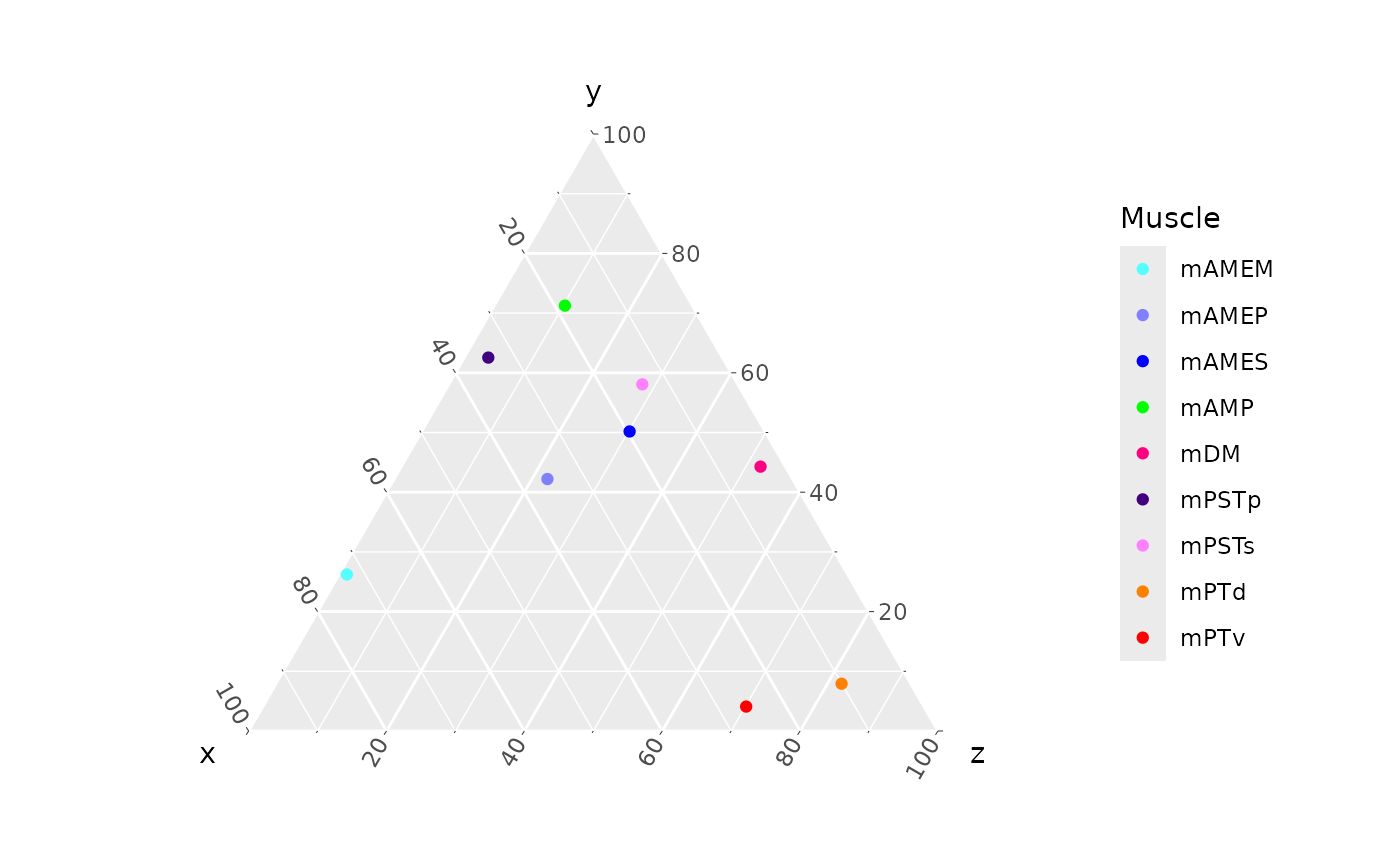
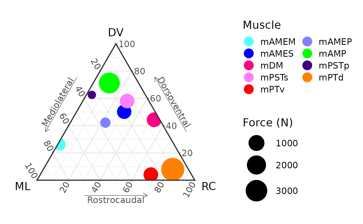
And finally we can add labels, change the theme, fix up the legend,
and update the scale, resizing the points according to
force. Points don’t have to be scaled to force, any proxy
for body size (SVL, head width, etc. would work as well).
ggtern(data = ternary_coords,
       aes(x = x, y = y, z = z,
           color = muscle,
           size = force)) +
  geom_point() +
  muscle_color_map() +
  labs(x       = "ML",
       xarrow  = "Mediolateral",
       y       = "DV",
       yarrow  = "Dorsoventral",
       z       = "RC",
       zarrow  = "Rostrocaudal") +
  theme_bw(base_size = 16) +
  theme_showarrows() +
  scale_size_continuous(range = c(5, 15), name = "Force (N)") +
  guides(colour = guide_legend(override.aes = list(size = 6),
                               ncol = 2, byrow = TRUE))
#> Ignoring unknown labels:
#> • xarrow : "Mediolateral"
#> • yarrow : "Dorsoventral"
#> • zarrow : "Rostrocaudal"