Carry out the Johnson-Neyman Technique
Details
| Package: | jnt |
| Type: | Package |
| Version: | 0.4 |
| Date: | 2016-09-14 |
| License: | GPL-2 |
| LazyLoad: | yes |
| LazyData: | yes |
References
Johnson PO, Neyman J (1936) Tests of certain linear hypotheses and their application to some educational problems. Statistical Research Memoirs 1:57-93.
Hunka S, Leighton J (1997) Defining Johnson-Neyman regions of significance in three-covariate ANCOVA using Mathematica. Journal of Educational and Behavioral Statistics 22: 361-387.
White CR (2003) Allometric analysis beyond heterogenous regression slopes: Use of the Johnson-Neyman Technique in comparative biology. Physiol Biochem Zool 76: 135-140.
Examples:
White CR (2003) The influence of foraging mode and arid adaptation on the basal metabolic rates of burrowing mammals. Physiol Biochem Zool 76: 122-134.
Lavin SR, Karasov WH, Ives AR, Middleton KM, Garland T, Jr (2008) Morphometrics of the avian small intestine compared with that of nonflying mammals: A phylogenetic approach. Physiol Biochem Zool 81: 526-550.
Author
Kevin Middleton (middletonk@missouri.edu)
Maintainer: Kevin Middleton (middletonk@missouri.edu)
Examples
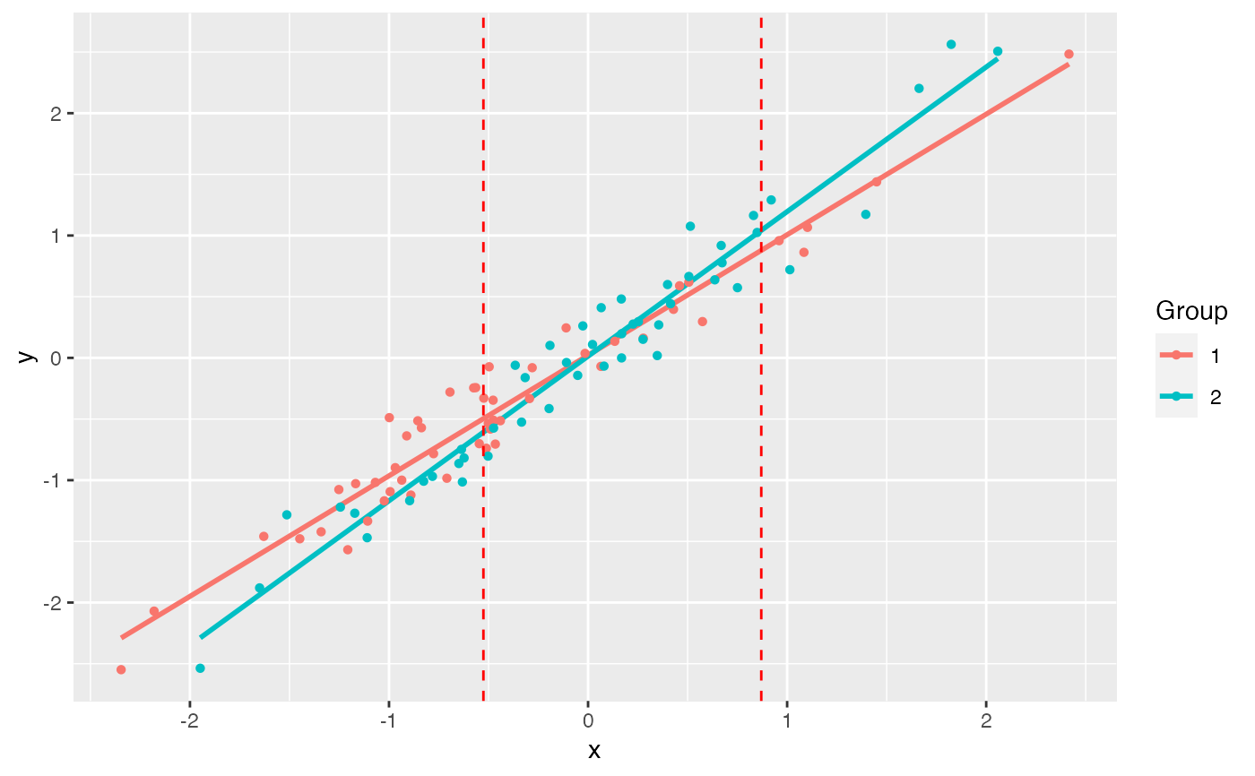
example(jnt)
#>
#> jnt> # Simulate data
#> jnt> set.seed(1234)
#>
#> jnt> n <- 50
#>
#> jnt> x1 <- rnorm(n)
#>
#> jnt> y1 <- x1 + rnorm(n, sd = 0.2)
#>
#> jnt> x2 <- rnorm(n)
#>
#> jnt> y2 <- 1.25 * x2 + rnorm(n, sd = 0.2)
#>
#> jnt> df1 <- data.frame(x = x1, y = y1)
#>
#> jnt> df2 <- data.frame(x = x2, y = y2)
#>
#> jnt> (jnt.out <- jnt(df1, df2))
#> Fitting with OLS
#> Assuming x variable is column 1, and y is column 2.
#>
#> Johnson-Neyman Technique
#>
#> Alpha =  0.05
#>
#> Data 1:
#> 	Slope		 0.9853
#> 	Intercept	 0.02126
#>
#> Data 2:
#> 	Slope		 1.182
#> 	Intercept	 0.01386
#>
#> Region of non-significant slope difference
#> 	Lower: -0.5258
#> 	Upper: 0.8701
#>
#>
#> jnt> plot(jnt.out)
#> `geom_smooth()` using formula 'y ~ x'