Data from White, 2003

Data set 1 from from White, 2003

Format

A data frame with 50 observations on the following 2 variables.

V1

a numeric vector

V2

a numeric vector

References

White CR (2003) Allometric analysis beyond heterogenous regression slopes: Use of the Johnson-Neyman Technique in comparative biology. Physiol Biochem Zool 76: 135-140.

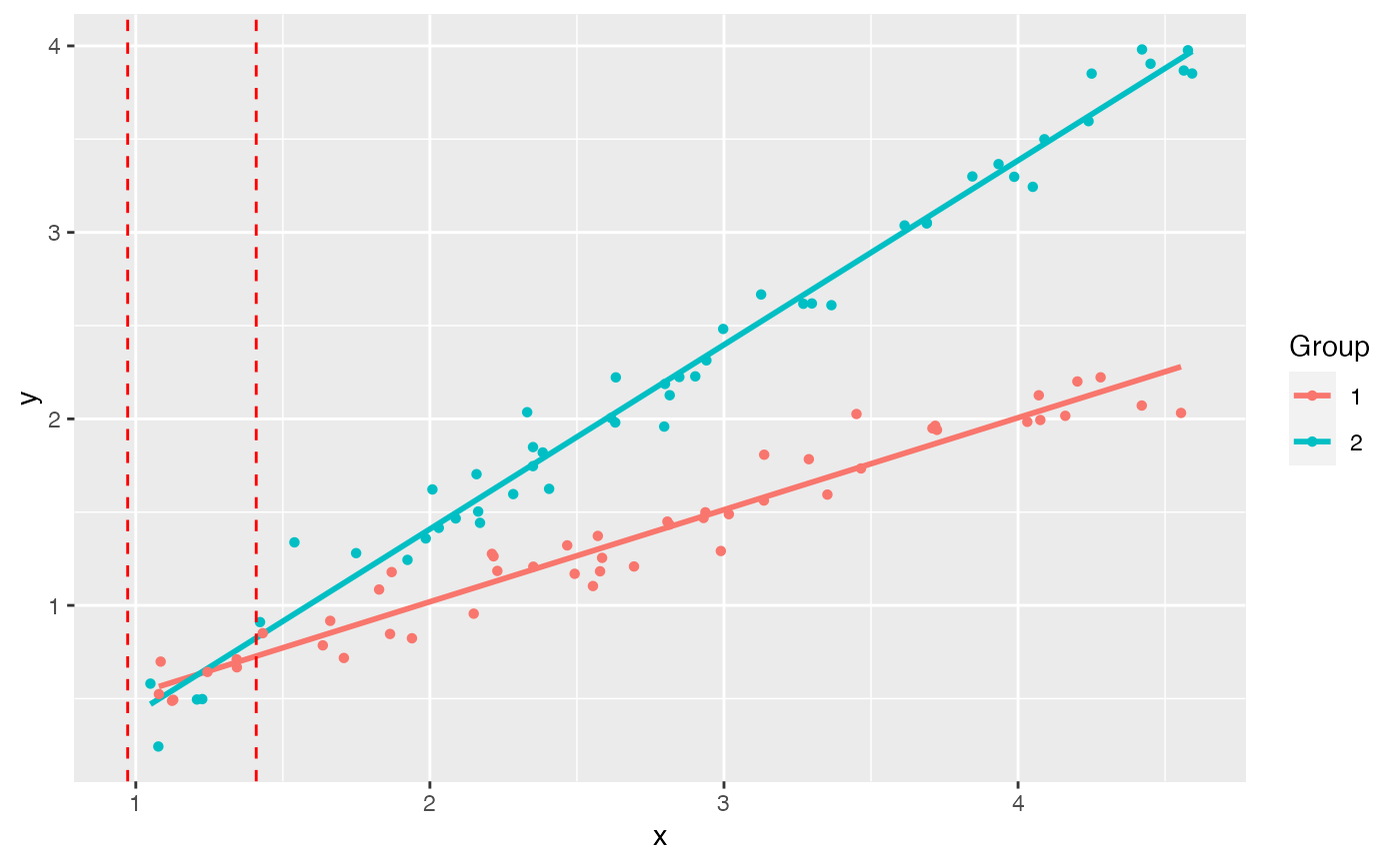
Examples

str(White.1)
#> 'data.frame':	50 obs. of  2 variables:
#>  $ V1: num  3.45 2.49 1.86 1.83 1.12 ...
#>  $ V2: num  2.026 1.169 0.847 1.085 0.488 ...
str(White.2)
#> 'data.frame':	50 obs. of  2 variables:
#>  $ V1: num  2.63 3 1.99 2.28 2.8 ...
#>  $ V2: num  1.98 2.48 1.36 1.6 2.19 ...

(White <- jnt(White.1, White.2))
#> Fitting with OLS
#> Assuming x variable is column 1, and y is column 2.
#> 
#> Johnson-Neyman Technique
#> 
#> Alpha =  0.05 
#> 
#> Data 1:
#> 	Slope		 0.4935 
#> 	Intercept	 0.03244 
#> 
#> Data 2:
#> 	Slope		 0.9883 
#> 	Intercept	 -0.5676 
#> 
#> Region of non-significant slope difference
#> 	Lower: 0.9724 
#> 	Upper: 1.41 
#> 
plot(White)
#> `geom_smooth()` using formula 'y ~ x'